Rasterize
Menu / Icon
This tool is accessible via the 'Tools > Projection > Rasterize' menu or the ![]() icon in the upper main toolbar.
icon in the upper main toolbar.
(Prior to version 2.6.1, this tool was named 'Height grid generation')
Description
The main purpose of this tool is to 'rasterize' a point cloud (i.e. convert it to a 2.5D grid) and then export it as a new cloud or a raster image (geotiff) for instance.
Another application since version 2.6.1 is 'Contour plot' generation.
Procedure
Select one cloud then start this tool.
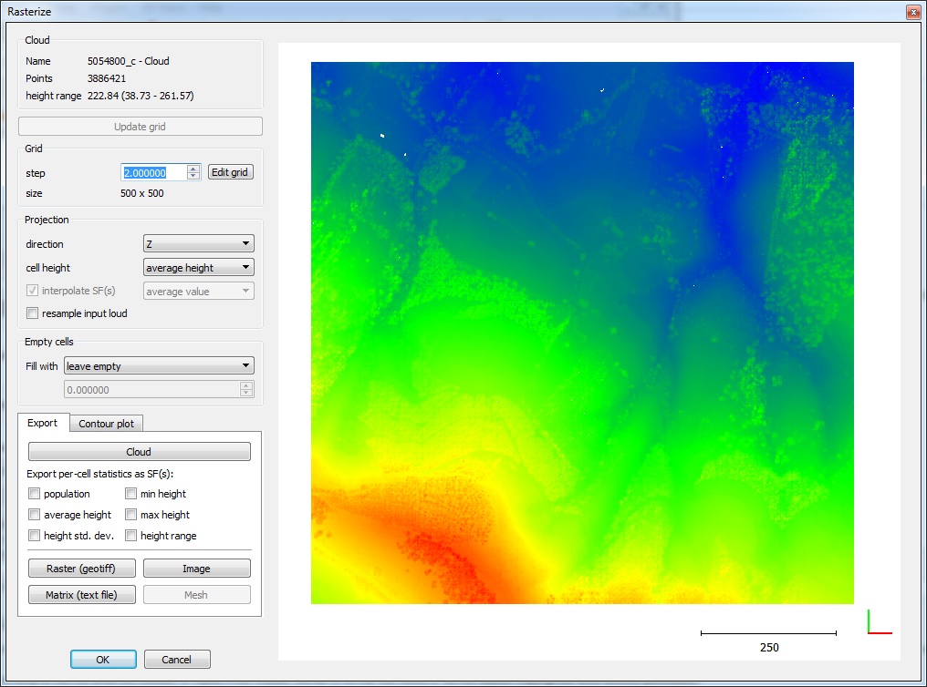
A dedicated dialog with an embedded 3D view will appear. Some pieces of information about the selected cloud are displayed in the upper-left corner. The most important is the height range and the minimum and maximum height values of the cloud (the height being considered along the projection dimension).
Generating a raster grid
The first and mandatory step is to generate the raster grid.
The user must define the main (raster) grid generation parameters:
- the grid step size (CloudCompare will update the resulting grid size below so that the user can check that the grid is neither too big nor too small before actually generating the grid)
- the projection direction (X, Y or Z - default: Z)
- how the 'height' of each cell grid will be computed:
- minimum value of all points falling in this cell
- average value of all points falling in this cell
- maximum value of all points falling in this cell
- since version 2.13:
- median value of all points falling in this cell
- inverse variance: the height or scalar value of each cell is equal to a weighted average of the points falling inside the cell. The weights are equal to the inverse variance (= 1/std_dev^2). Standard deviation values (std_dev) are obtained from an already existing scalar field, which must be selected by the user.
- since version 2.6.2 the user can choose the 'active layer' that will be projected. The default layer is 'height grid values' (i.e. the coordinate of the points along the projection dimension) but it can now be any scalar field associated to the selected cloud, the hillshade layer, etc.
Once the base parameters are properly set, the user must click on the 'Update grid' button to make CloudCompare actually compute the grid and display it.
Each time a parameter is modified, the 'Update grid' button will appear in red. The user has to click on it to actually apply the changes.
Advanced parameters
Empty cells
If no point falls inside a given cell, this cell will be considered as 'empty'. By default empty cells are not visible when displayed in the tool's 3D view. They generally have a dedicated 'NaN' or 'empty' value when exported to a raster file (depending on the format).
It is possible to fill these cells in various ways:
- use the minimum height of the whole grid
- use the average height of the whole grid
- use the maximum height of the whole grid
- use a user specified value (should be input in the field below the 'Fill with' drop-down list)
- interpolate (see below)
Interpolating empty cells
Interpolate
The 'interpolate' option consists in a linear interpolation with the nearest non-empty neighboring cells. It relies on Delaunay triangulation.
This can give very good results in the presence of small holes. However it can be less realistic on large holes. The biggest limitation is that it's limited to the convex hull of the non-empty cells. Therefore a custom/default value must still be specified in the field below the 'Fill with' drop-down list to fill the remaining empty areas (if any).
Kriging
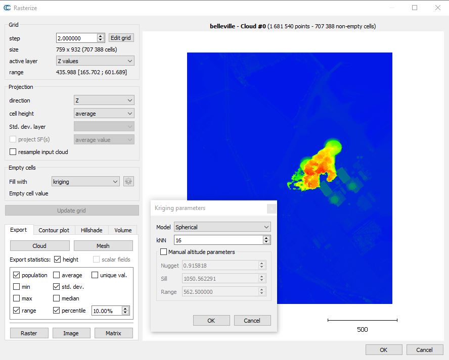
It is now possible to use a Kriging algorithm to fill the empty cells. While this option may take more time to compute, it allows to interpolate cells all over the raster grid and not only inside the non-empty cells convex hull.
Grid position
The grid position (in the projection plane) can be finely defined by clicking on the 'Edit grid' button:
Warning: the Rasterize tool grid uses the 'pixel-is-area' convention but the grid itself is centered on the boundary pixel centers. The grid min corner coordinates correspond to the lower left raster cell center, and the grid max corner coordinates correspond to the upper right raster cell center:
Interpolate scalar fields
If the input cloud has one or several scalar fields, it is possible to 'interpolate' the scalar field values in each grid cell.
To do this the user has to check the 'interpolate SF(s)' checkbox and define how this interpolation should be conducted:
- by keeping the minimum SF value of all the points falling in this cell
- by keeping the average SF value of all the points falling in this cell
- by keeping the maximum SF value of all the points falling in this cell
- since version 2.13:
- median value
- inverse variance
Note: interpolated scalar fields can only be used when exporting the raster grid as a new cloud or as a raster file in a formats that supports real-valued layers.
Resample input cloud
This option tells CloudCompare to keep in each grid cell the point from the input cloud which is the closest to the cell center (instead of the cell center itself). This way it is possible to subsample the cloud in a semi-gridded pattern. If the grid is to be exported as a cloud, all the input cloud features (colors, normals, etc.) can be properly exported as well.
Since version 2.7 the resample option can now be used with the 'average height' projection. In this case only the 2D coordinates of the original point are kept (the point which is the closest to the cell center) and the height is replaced by the average cell height.
Export
The (raster) grid can be exported to several destinations.
Cloud
The grid can be exported as a new cloud (see the "Cloud" button in the 'Export' tab in the bottom-left corner).
The grid is always exported as a 3D cloud (with the chosen 'height' as the 'Z' dimension). A 'height' scalar field is also generated by default.
Several additional scalar fields can be generated:
- 'population': number of input points falling in each cell
- 'min': minimum height of the points falling in each cell
- 'average': average height of the points falling in each cell (may be redundant with the default 'height' scalar field)
- 'max': maximum height of the points falling in each cell (may be redundant with the default 'height' scalar field)
- 'std. dev.': standard deviation of the height values of the points falling in each cell
- 'range': range of the height values of the points falling in each cell
- Since version 2.13:
- 'unique val.': the number of uniques values inside each cell
- 'median': median value
- 'percentile' + percentage: highest value of the given percentage of points (sorted)
Since version 2.13, it is now also possible to choose whether the above statistics should be applied to 'height' values, all the 'scalar fields' or both (with checkboxes).
Raster
The grid can be exported as a geotiff raster file (see the "Raster (geotiff)" button in the 'Export' tab in the bottom-left corner).
Note: CloudCompare relies on GDAL for this operation.
Image
The grid can be exported as a simple image file. Use the 'Image' button (see the "Image" button in the 'Export' tab in the bottom-left corner).
ASCII matrix
The grid can be exported as an array/matrix of height values saved as an ASCII file (see the "Matrix (text file)" button in the 'Export' tab in the bottom-left corner).
This file should be easily imported in Excel for Matlab for instance. There's no file header. The number of rows is simply the number of lines in the file, and the number of columns corresponds to the number of values found on each line (should always be the same).
Mesh
The grid can be exported as a 2.5D mesh (see the "Mesh" button in the 'Export' tab in the bottom-left corner).
Contour plot generation
Since version 2.6.1, the Rasterize tool can now be used to generate contour plots.
The parameters for this sub-tool are all regrouped in the 'Contour plot' tab in the bottom-left part:
The user must specify:
- Start height: height of the first contour line
- Step: step between each contour line
- Min. vertex: minimum number of vertices per lines (used to remove the very small contours around trees, etc.)
- ignore borders: to remove the contour lines created on the grid (square) edges
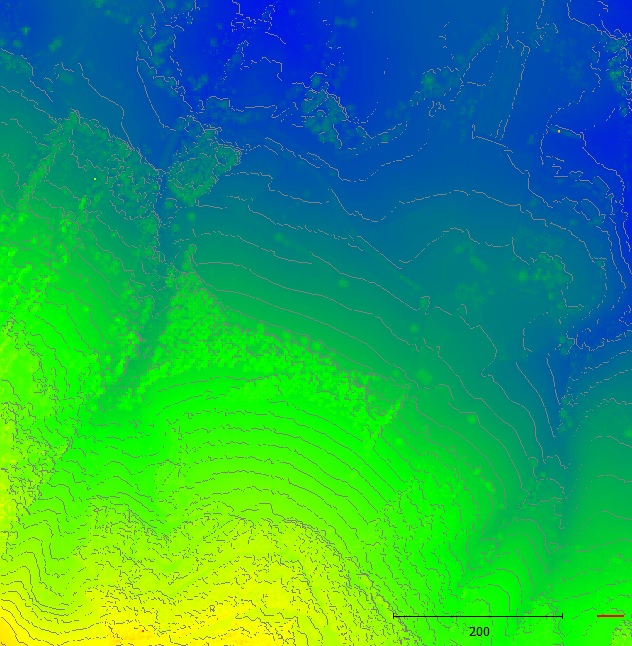
The first time, and each time the parameters are changed or the grid is updated, the user must click on the 'Generate' button to generate the contour plot. Then a preview of the generated contour lines will be displayed over the raster grid:
The user can pan and zoom the 3D view to view it better. The point size can also be modified in the standard way (+/- interactors appear when the mouse hovers the top-left part of the 3D view).
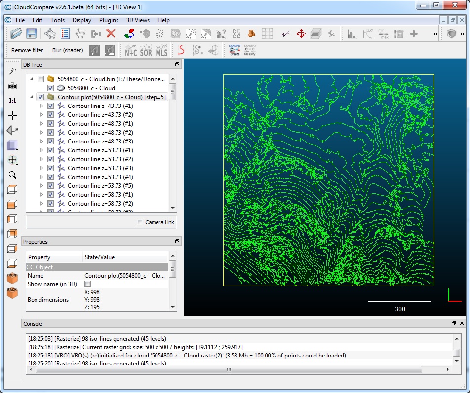
The resulting contour lines can be removed (with the 'Clear' button) or exported as real polylines in the DB tree (with the 'Generate' button). All contour lines are exported in a single group (automatically named after the input cloud name and the 'Step' value).
Notes:
- the (group of) contour lines can be exported as a Shape file (to be imported in a GIS software for instance).
- if the user has forgotten to export the contour lines when closing the tool, CloudCompare will issue a warning message and will ask for confirmation.
Since version 2.6.2
- the 'active layer' is used to compute the contour lines (this way contour lines can be computed on any scalar field)
- the default width of contour lines can be set prior to generating them
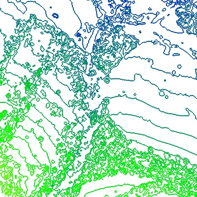
- the contour lines can be colored based on their height (with the active layer color ramp) - use the 'colorize' check box
Hillshade
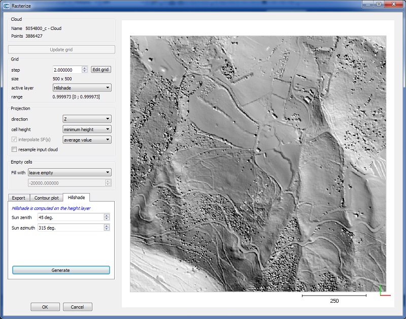
Since version 2.6.3, the Rasterize tool can generate an hillshade layer:
Once the grid has been generated:
- click on the 'Hillshade' tab
- set the right parameters (sun position)
- click on generate
Note that this layer will disappear each time the 'Update grid' button is clicked
