Cloud-to-Cloud Distance
Menu / Icon
This tool is accessible via the ![]() icon in the main upper toolbar or the 'Tools > Distances > Cloud/Cloud dist.' menu.
icon in the main upper toolbar or the 'Tools > Distances > Cloud/Cloud dist.' menu.
Description
This tool computes the distances between two clouds.
Procedure
To launch this tool the user must select two clouds (and only two).
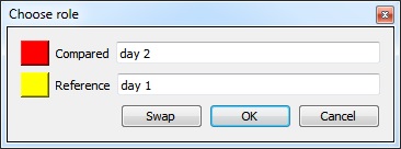
Choosing the cloud roles
Before displaying the tool dialog, CloudCompare will ask you to define the roles of each cloud:
- the Compared cloud is the one on which distances will be computed. CloudCompare will compute the distances of each of its points relatively to the reference cloud (see below). The generated scalar field will be hosted by this cloud.
- the Reference cloud is the cloud that will be used as reference, i.e. the distances will be computed relatively to its points. If possible, this cloud should have the widest extents and the highest density (otherwise a local modelling strategy should be used - see below).
Approximate distances
When the Cloud/Cloud distance computation dialog appears, CloudCompare will first compute approximate distances (which are used internally to automatically set the best octree level at which to perform the real distances computation - see below). The reference cloud is hidden and the compared cloud is colored with those approximate distances.
Some statistics on those approximate distances are displayed in the 'Approx. results' tab (but they shouldn't be considered as proper measurement values!). Those statistics are only provided for advanced users who would like to set the octree level at which computation is performed themselves (however this is generally not necessary).
The user must compute the real distances (see the red 'Compute' button) or cancel the process.
Parameters
The main parameters for the computation are:
- Octree level: this is the level of subdivision of the octrees at which the distance computation will be performed. By default it is set automatically by CloudCompare and should be left as is. Changing this parameter only changes the computation time. The main idea is that the higher the subdivision level is, the smaller the octree cells are. Therefore the less points will lie in each cell and the less computations will have to be done to find the nearest one(s). But conversely, the smaller the cells are and the more cells may have to be searched (iteratively) and this can become very slow if the points are far apart (i.e. the compared point is far from its nearest reference point). So big clouds will require high octree levels, but if the points of the compared cloud are rather far from the reference cloud then a lower octree level is better...
- Max dist.: if the maximum distance between the two clouds is high, the computation time might be awfully long (as the farther the points are, the more time it will take to determine their nearest neighbors). Therefore it can be a good idea to limit the search below a reasonable value to shorten the computation time. All points farther than this distance won't have their true distance computed - the threshold value will be used instead.
- signed distances: not available for cloud-to-cloud distance.
- flip normals: not available for cloud-to-cloud distance.
- multi-threaded: whether to use all CPU cores available (warning: the computer might not be totally responsive during the computation)
- split X,Y and Z components: generate 3 more scalar fields corresponding to the (absolute) distance between each compared point and its nearest reference point along each dimensions (i.e. this corresponds to the 3 components of the deviation vector).
Local modelling
(see the 'Distances Computation' section for additional information)
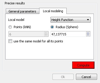
When no local model is used, the cloud to cloud distance is simply the nearest neighbor distance (using a kind of Hausdorff distance algorithm). The issue is that the nearest neighbor is not necessarily (rarely in fact) the actual nearest point on the surface represented by the cloud. This is especially true if the reference cloud has a low density or has big holes. In this case it can be a good idea to use a 'Local modelling strategy' which consists in computing a local model around the nearest point so as to approximate the real surface and get a better estimation of the 'real' distance.
The local model can be computed:
- either on a given number of neighbors (this is generally faster but it's only valid for clouds with a constant density)
- or by default in a spherical neighborhood (its radius should typically depend on the details you expect to catch and on the cloud noise).
There are currently three types of local models. All 3 models are based on the least-square best fitting plane that goes through the nearest point and its neighbors:
- Least squares plane: we use this plane directly to compute distances
- 2D1/2 triangulation: we use the projection of the points on the plane to compute Delaunay's triangulation (but we use the original 3D points as vertices for the mesh so as to get a 2.5D mesh).
- Quadric (formerly called 'Height function'): the name is misleading but it is kept for consistency with the old versions. In fact the corresponding model is a quadratic function (6 parameters: Z = a.X2 + b.X + c.XY + d.Y + e.Y2 + f). In this case we only use the plane normal to choose the right dimension for 'Z'.
We could say that the local models are sorted in increasing 'fidelity' to the local geometry (and also by increasing computation time). One should also take in consideration whether the local geometry is mostly smooth or with sharp edges. Because the Delaunay triangulation is the only model that can theoretically represent sharp edges (assuming you have points on the edges) and the quadratic function is the only one that can represent smooth/curvy surfaces. By default it is recommended to use the quadratic model as it's the more versatile.
Last but not least it's important to understand that due to the local approximation, some modeling aberrations may occur (even if they are generally rare). The computed distances are statistically much more accurate but locally some distance values can be potentially worse than the nearest neighbor distance. This means that one should never consider the distance of a single point in its analysis but preferably a local tendency (this is the same with nearest neighbor distance anyway). To partially cope with this effect, since version 2.5.2 we now keep for each point the smallest distance between the nearest neighbor distance and the distance to the local model. This way, we can't output distances greater (i.e. worst) than the nearest neighbor's one. However we can still underestimate the 'true' distance in some (hopefully rare) cases.
The 'local modeling' strategy is meant to cope with sampling-related issues (either a globally too small density or too high local variations of the density of the reference cloud). It's always a good idea to use the densest cloud as 'reference'.
Displaying the resulting distances color scale
Once the computation is done, the user can close the dialog. To display the resulting scalar field's color scale, just select the compared cloud and then check the 'Visible' checkbox of the 'Color Scale' section of its properties.
Alternatively use the shortcut 'Shift + C' once the cloud is selected to toggle the color scale visibility.
One can also set the color scale to be used with the 'Current' combo-box (and edit it or create a new one with the 'gear' icon on the right).


